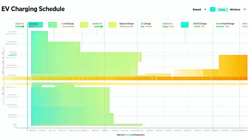
Demand charges are the line item that makes commercial EV charging economics brutal. At many US utilities on commercial rates, demand charges — billed on the peak 15-minute interval in a billing cycle — can represent 40 to 60 percent of total electricity cost for a depot charging operation. A fleet that draws 500 kW for one 15-minute window at 3 PM on a weekday, then charges the rest of the month at off-peak, pays as though it ran 500 kW for the entire month.
The math is simple. The execution — knowing exactly which windows are off-peak, what the grid congestion signal looks like at a given site, and dispatching charging to stay below a demand threshold — requires real-time data and automated decision logic. This article walks through the API workflow to build that logic using Derapi's load management endpoints.
Why Demand Charge Reduction Compounds
A growing EV fleet operation in the Pacific Northwest, operating 30 electric delivery vehicles out of a depot in the Portland metro area, illustrates the compounding dynamic well. The site has a 750 kW utility service connection. Without load management, vehicle charging at end-of-shift (typically 4–7 PM) creates a demand peak coinciding with the grid's own evening ramp. PGE's commercial Schedule 746 includes demand charges in the $12–$18/kW range depending on the season. A 400 kW demand peak means roughly $4,800–$7,200 in demand charges alone — per month.
Shift the same charging load to 10 PM–4 AM, when the vehicles aren't in service and grid demand is low, and the demand peak from the fleet drops to near zero (the site's baseline HVAC and facility load sets the demand). The vehicles still receive a full charge. The demand charge line item collapses. The 40% figure in the article title is achievable in this scenario because demand charges are the dominant cost element; flattening the peak means eliminating a category of cost, not just reducing it proportionally.
The Grid Congestion Signal: What Derapi Returns
Intelligent charge scheduling requires two inputs: knowledge of when charging is cheapest (or least grid-stressed) and knowledge of each vehicle's state of charge (SoC) and required departure time. The second input comes from your fleet management system. The first comes from the grid.
Derapi's grid congestion endpoint returns a forward-looking congestion signal for the utility territory serving a given location:
GET /v1/grid/congestion?zip=97202&horizon=24h&interval=15mThe response includes a congestion_score (0.0–1.0, where 0.0 is uncongested and 1.0 is maximum stress), a price_signal in $/kWh for utilities that publish real-time or day-ahead locational marginal prices (LMPs), and a recommended_charge_windows array — sorted by congestion score, lowest first — showing the optimal 15-minute intervals in the requested horizon.
For utilities without LMP data (most distribution-level utilities don't publish LMPs), Derapi derives the congestion signal from publicly available load forecasts, temperature data, and historical demand patterns. The score is an approximation, not an LMP. Your application should indicate this distinction to operators who may assume price precision that the data doesn't support.
Building the Scheduling Decision Loop
The scheduling workflow looks like this at a high level:
- At the start of each scheduling horizon (e.g., 4 PM daily), query the congestion endpoint for the next 24 hours at 15-minute intervals.
- Pull each vehicle's current SoC and required departure time from your fleet management API.
- Calculate the minimum energy (kWh) needed per vehicle:
(target_soc - current_soc) × battery_capacity_kwh. - Rank charging windows by congestion score (ascending). Assign charging slots to the lowest-congestion windows that have sufficient time before each vehicle's departure.
- Apply the demand threshold constraint: sum the scheduled charging load across all vehicles in each 15-minute interval, and ensure no interval exceeds the site's demand target (e.g., 80% of contracted capacity to leave headroom).
- Dispatch charging instructions to each EVSE via your charging network management system (CNMS) API.
- Re-run the loop hourly or when SoC deviates significantly from the model (e.g., a vehicle returns early with lower-than-expected SoC).
This loop is not complex to build. The hard part historically was step 1 — getting reliable, machine-readable congestion or price signals for the utility territory. That's the gap Derapi fills.
Rate Structure Considerations: TOU, Demand, and NEM
Not all utilities structure commercial EV charging rates the same way, and the correct optimization target depends on the rate schedule. Derapi's rate lookup endpoint returns the applicable tariff for a given utility account or service address:
GET /v1/utility/rate?zip=97202&customer_class=commercial&load_type=ev_chargingThe response includes the rate schedule name, the time-of-use (TOU) windows if applicable (on-peak, mid-peak, off-peak hour ranges), the demand charge structure ($/kW, measured on 15-minute or 30-minute intervals), and any EV-specific riders or optional rates the utility offers.
We're not saying demand charge reduction is the only lever worth optimizing. For utilities with steep TOU differentials — some California IOUs have on-peak vs. off-peak rate spreads of $0.20–$0.30/kWh — pure energy arbitrage (charge in off-peak hours) can produce comparable savings to demand charge reduction, especially for lower-throughput depots where the demand peak is modest. Your application should calculate both effects separately and optimize for total cost, not just demand.
If the site has behind-the-meter solar and battery storage, the optimization problem expands: now you're also deciding whether to charge EVs from the battery (discharging it) or from the grid, based on what the battery is worth for demand response or grid services. That's a third-order problem. Derapi returns the grid signal; your application's dispatch logic decides the stack ranking among grid charging, battery discharge, and solar generation.
V2G Eligibility and Interconnect Status
Vehicle-to-grid (V2G) capability — where EVs export stored energy back to the grid or to facility loads — adds another dimension to the scheduling problem. A V2G-capable vehicle is both a load and a potential resource. During a high-congestion window, a fleet with V2G support might dispatch partial discharge instead of curtailing charging: export 50 kW from vehicles with high SoC, reducing net grid draw during the peak period.
Derapi's EVSE interconnect endpoint includes a v2g_eligible flag for the utility territory and a v2g_program field pointing to any active utility V2G pilot or program that the site may qualify for. As of early 2025, utility V2G programs are still largely in pilot phase in the US, with several California and Pacific Northwest utilities running active managed charging and V2G demonstration programs. The eligibility data is updated as programs expand or close enrollment.
Your application should not assume V2G is available everywhere your fleet operates. Check the flag per site. Where V2G is eligible, surface it to the operator as an optional optimization mode — the potential revenue from grid services can partially offset the cost of charging, but it also increases battery cycle count, which has a cost that your model should account for.
The 40% Figure in Context
Demand charge savings of 30–45% are well-supported in the published literature for managed charging deployments at commercial depots. The range depends heavily on the baseline behavior (unmanaged end-of-shift charging), the rate structure, and the fleet's flexibility window (vehicles that must depart at 6 AM have a narrower charging window than vehicles with flexible overnight dwell time).
A 40% reduction in total electricity cost is achievable when demand charges represent a majority of the bill and when the fleet has a wide charging flexibility window — typically 8+ hours of dwell time overnight. Depots with vehicles that do multiple shifts, short dwell times, or unpredictable return times have less flexibility, and the optimization upside shrinks accordingly.
Building the scheduling logic described here requires the grid signal, the rate structure, and the fleet SoC data to be available in a single coherent data model. The Derapi endpoints provide the first two. Connect them to your fleet system's SoC telemetry and you have everything needed to run the loop.